…Or, can we trust these estimates?

One of the most common questions that comes up in scientific publications is “Can I trust these conclusions?” Statistics is supposed to help us decide the weight of evidence for or against a certain conclusion, but there have been issues. We are realizing that the standard paradim is not holding up, and there are many more false positives in the literature than the p < 0.05 cutoff would have us believe. A large issue is that under-powered studies can result in estimates which are too large (magnitude or Type M errors) or are the opposite sign (sign, or Type S errors). Or, when we are interested in the difference between two treatments, an underpowered study will no be able to detect the effect.

One way to resolve these issues and determine how much trust you should put into a piece of work is to conduct a retroactive power analysis.

What is “power”?

Power is a measure of how likely we are to find an effect. Our chances of detecting an effect is affected by many factors:

• The effect size: Larger effects are easier to find
• The variation between samples (i.e., the error): Less noise or variation makes effects easier to detect
• Sample size: the more observations we have, the more certain we are of the estimate

Why conduct a power analysis after the fact?

There are many good reasons. A power analysis can tell you how large of an effect the study could reliably detect. It is too common for p > 0.05 to be interpretted as “no difference between treatments” or “no effect”, but many of those studies were under-powered and never had a chance to detect the effect. On the other side of the coin, when one finds a significant effect in an underpowered study, odd are that either the sign of the estimate or the magnitude is wrong (or even both).

Example: Typical agricultural experiment

For this example, I am going to use this paper by Carrijo et al., 2018. I am using this paper because I am familiar with the system, have auxiliary data to leverage, and it is open access so anyone can follow along. To be clear, this is just one example - similar examples can be found throughout the scientific literature.

That said, this paper is prime example of where a lack of statistical significance was interpretted as “no difference” rather than the more accurate “the difference was smaller than our power to detect”. So, what size of effect size could they have detected?

Note: although there are packages which can do this more or less automatically, we will do it “by hand” for demonstration purposes.

First, we need to know the experimental design. The authors report a 2 year experiment with a randomized complete block design with 3 replications and 3 treatments in 2015 and 4 in 2016.

Now, how were the data analyzed? The authors report a within year (i.e., each year was modeled separately) linear model with block and treatment as fixed effects.

If you just did a double take, then good on you. There are already issues in the analysis. We will look at the original analysis and as well as a more robust one in a later post.

The last pieces we need are some estimate of magnitude of variation within treatments. We will use a rough estimate based on the numbers as reported by the authors to start. Specifically, we are going to assume the variation between treatments is shared.

Now, we don’t have access to the original data, so we are going to have to do some estimating for the standard deviation within treatments. To do this, we are going to change the the standard deviation and will see how different levels of variation affect our power.

From a previous meta-analysis by these same authors, we expect a roughly 5–10% effect size. Taking yield as an example, based on the tables in the paper, we can estimate that the average yield to be around 11 Mg/ha, which makes the a priori estimate of the effect 0.55 – 1.1. That is, we expect the AWD treatment to decrease yields by 0.55–1.1 Mg/ha

intercept = 11
beta_treatment = c(0, -0.55, -1.1)

Getting the error is a little more difficult. The standard errors reported range from 0.08 to 0.48. But this will include both block to variation as well as the within treatment variation. We will work with the optimistic assumption that the blocks have a low variance.

Since we are not really interested in the blocks, we are just going to set them with roughly a standard deviation of 0.075 and arrange them so that their effects sum to zero,

beta_block = c(0.15, 0, -0.15)

As we will see, the model assumes a shared error term for all observations. In other studies working at this same site, I have estimated the measurement error to be roughly 0.9 Mg/ha. If we are optimistic that the standard error is lower here, we can get an estimate of the measurement error from the standard errors reported (standard error = \( \sigma / \sqrt{n} \) ). Based on the numbers reported in the paper and this equation, we will use 0.34 Mg/ha (very optimistic based on other data from this site).

sigma = 0.34

Now, we can set up our simulation framework.

Defining the data generative process

Ok, now that we have set the of the experiment variables, we need to make a function that defines the data generative model. What does that mean? Well, our statistical analysis assumes the data are being generated in a certain way. We want to mimic that in order to generate some fake data.

Since the authors state they used a simple linear model, we know the mean variable is assumed to be a linear function of the form:

$$ y_{ij} = intercept + \beta_{treatment\ i} + \beta_{block\ j} + \epsilon $$

We need to convert this into a function which produces random data when called, and takes the parameters as inputs. Since we want this to produce random data, we have two choices:

1. we can provide a fixed set of betas, and then the only randomness is from the error term,
2. we can allow the betas to vary within a range

Since the first generally aligns with the frequentist interpretation of parameters, we will use that one. We will use the fixed estimates for beta defined earlier.

Now we will define a function to simulate data,

simulate_data = function(intercept,
                         beta_treatments,
                         beta_blocks,
                         sigma)
{
    n_treat = length(beta_treatments)
    n_block = length(beta_blocks)
    data_matrix = expand.grid(treatment = seq(n_treat),
                              block = seq(n_block))
    data_matrix$mu = intercept +
        beta_treatments[data_matrix$treatment] +
        beta_blocks[data_matrix$block]

    data_matrix$y = rnorm(nrow(data_matrix), data_matrix$mu, sigma)
    
    return(data_matrix)
}

Next, we want to generate a bunch of random datasets and figure out how often we are able to detect a significant effect.

Again, we are going to make a function to do this,

power_analysis = function(intercept,
                          beta_treatments,
                          beta_blocks,
                          sigma,
                          alpha = 0.05)
{
    d = simulate_data(intercept,
                      beta_treatments,
                      beta_blocks,
                      sigma)
    mod = aov(y ~ factor(treatment) + factor(block), data = d)
    
    # p-value for treatment - logical
    summary(mod)[[1]]$`Pr(>F)`[1] < alpha
}

and then we will replicate that a bunch of times, say 1000 using the values we established earlier,

table(replicate(1000,
                power_analysis(intercept,
                               beta_treatment,
                               beta_block, sigma)))

## 
## FALSE  TRUE 
##   331   669

You can see, this study has much lower then the standard 80% power, even with very optimistic assumptions about the measurement error. What if we use a still optimistic but more realistic measurement error of 0.5 Mg/ha?

table(replicate(1000,
                power_analysis(intercept,
                               beta_treatment,
                               beta_block, sigma = 0.5)))

## 
## FALSE  TRUE 
##   641   359

It becomes appearant that this study did not have good chances of detecting an effect in this system. Hence, the conclusion of “no difference” is suspect.

Put another way, the correct conclusion from these authors’ analysis is that the effect, if any, is smaller than their power to detect.

What effect size can they reliably detect?

The natural next question is how large of an effect can this study reliably detect?

We can answer this using the same framework above. Again, we will assume a optimistic 0.5 Mg/ha error - approximately half of the average error for experiments at this site.

We will test a range of effect sizes ranging from -0.25 to -3.5 Mg/ha,

beta_base = c(0, 0.5, 1)
beta_range = seq(0.25, 3.5, by = 0.25) * -1
test_cases = lapply(beta_range, `*`, beta_base)

ans = lapply(test_cases, function(x)
    table(replicate(1000,
                    power_analysis(intercept,
                                   beta_treatment = x,
                                   beta_block, sigma = 0.5))))
ans = as.data.frame(do.call(rbind, ans)/10)
colnames(ans) = c("No effect", "Effect")

and then we can plot the results,

plot(ans$Effect ~ beta_range, type = "b",
     xlab = "Effect size (Mg/ha)",
     ylab = "Power (%)")
abline(h = 80, lty = 2)

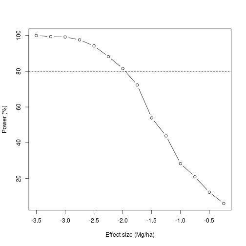
We can see that for this experiment to detect an effect with 80% power, the effect has to be approximately -2.0 Mg/ha, or 18% of yield – 3 times the estimated effect size from these authors’ previous work.

Now, a >10% drop in yield is sufficient to hurt a farmer’s bottom line, but here the authors conclude no effect. Knowing that there could have been up to a 18% decrease in yield and this study would not have been likely to detect it, we should recommend caution applying these treatments.

Conclusions

Here, with some straightforward R code, we have seen how retroactive power analysis can help us evaluate the support behind conclusions made in a scientific study. In this case, it seems unlikely that the study could detect the effect of interest.

Please note, as I said previously, I am not picking on this work or these authors. These issues exist in many published papers. This paper just happens to be a good example.